Julia数据科学系列-Makie

Makie.jl

Makie 基础教程

Makie的渲染后端

  • GLMakie: 交互式、3D渲染, 不能进行矢量图输出

  • CairoMakie: 矢量图输出, 高质量的2D图形, 不能3D渲染, 不能进行交互

  • WGLMakie: 网络端口, 类似GLMakie

julia

# 每种渲染方式都配套一个activate!()函数, 可以用于切换:
using CairoMakie
CairoMakie.activate!()

julia

Figure

  • Makie中最重要的对象是Figure, Axisplots

  • Figure命令定义一个画布(canvas), 在上边可以添加Axis, Colorbar, Legend等。

julia

f = Figure(
    backgroundcolor = :tomato, # 设置背景色
    resolution = (800, 300) # 设置分辨率

julia

Axis

julia

f = Figure()
ax = Axis(f[1,1],
    title = "title",
    xlabel = "x",
    ylabel = "y"
)
f

julia

Plots

定义好Figure和Axis后就可以把基础图形添加到Axis中:

julia

f = Figure()
ax = Axis(f[1, 1])
x = range(0, 10, length=100)
y = sin.(x)
lines!(ax, x, y)
f

julia

隐式调用Figure和Axis的基本函数

  • 基本绘图函数通常都包含两个版本, 一个加!, 一个不加: lines! 和 lines

  • 加叹号的会在现有Axis的基础上修改, 而不加叹号的版本(下称"无叹")会自动先创建Figure再定义Axis再把图画上:

julia

x = range(0, 10, length=100)
y = sin.(x)
lines(x, y) # 返回类型是FigureAxisPlot

julia
  • 所以无叹的基础绘图函数会返回一个元组: (Figure, Axis, Plot)

ind{\julia{ fig, axis, lineplot = lines(x, y) }}

  • Figureaxis也可以以关键字参数的形式在绘图函数中定义:

julia

scatter(x, y; 
    figure = (; resolution = (400, 400)),
    axis = (; title = "Scatter plot", xlabel = "Xs")
)

julia
Note 语法(; opt=xxx)中的;没有特别意义, 只是用来表示之后的变量是
  • 绘图函数有不同的调用方式:

julia

lines(x, y) # 基本的调用: 两个array
lines(1..10, sin) # 用函数生成y

julia

参数转换

x和y坐标可以是:

  • 具体的array: lines(0:10, 0:10)

  • 也可以是区间和转换函数: lines(0..10, sin)

  • 也可以是基本绘图元素的集合:

julia

# Points类型来自GeometryBasics.jl, 支持Makie中的大多数集合基本元素操作:
lines([Point(0, 0), Point(5,10), Point(10, 5)])

julia
不同图形支持的基本绘图元素集合是不一样的, 比如linesscatter都具有PointBased转换特征, 但heatmap就不能用Point, 因为需要的是2d-grid数据, 对应的特征是DiscreteSurface

图层和多图

!的函数会在原始图片的基础上添加新的图层进行绘制:

julia

x = range(0, 10, length=100)
f, ax, l1 = lines(x, sin)
l2 = lines!(ax, x, cos)
l2 = lines!(x, cos) # 可以省略axis的参数, 默认会用`current_axis()`函数获取当前的axis

julia

!的函数不能接受figureaxis关键字(of course!)

属性

  • 每个绘图函数都可以通过关键字参数设置不同的属性。

  • 还可以用plot.attribute = new_value这种语法来操作属性:

julia

x = range(0, 10, length=100)
f, ax, sc1 = scatter(x, sin, color = :red, markersize = 5)
sc2 = scatter!(ax, x, cos, color = :blue, markersize = 10)
f
# 改变属性
sc1.color = :yellow
sc2.strokewidth = 1
f # changed

julia
  • 属性可以设置成单个值, 也可以是数组(要与绘图元素等长)

Subplot子图

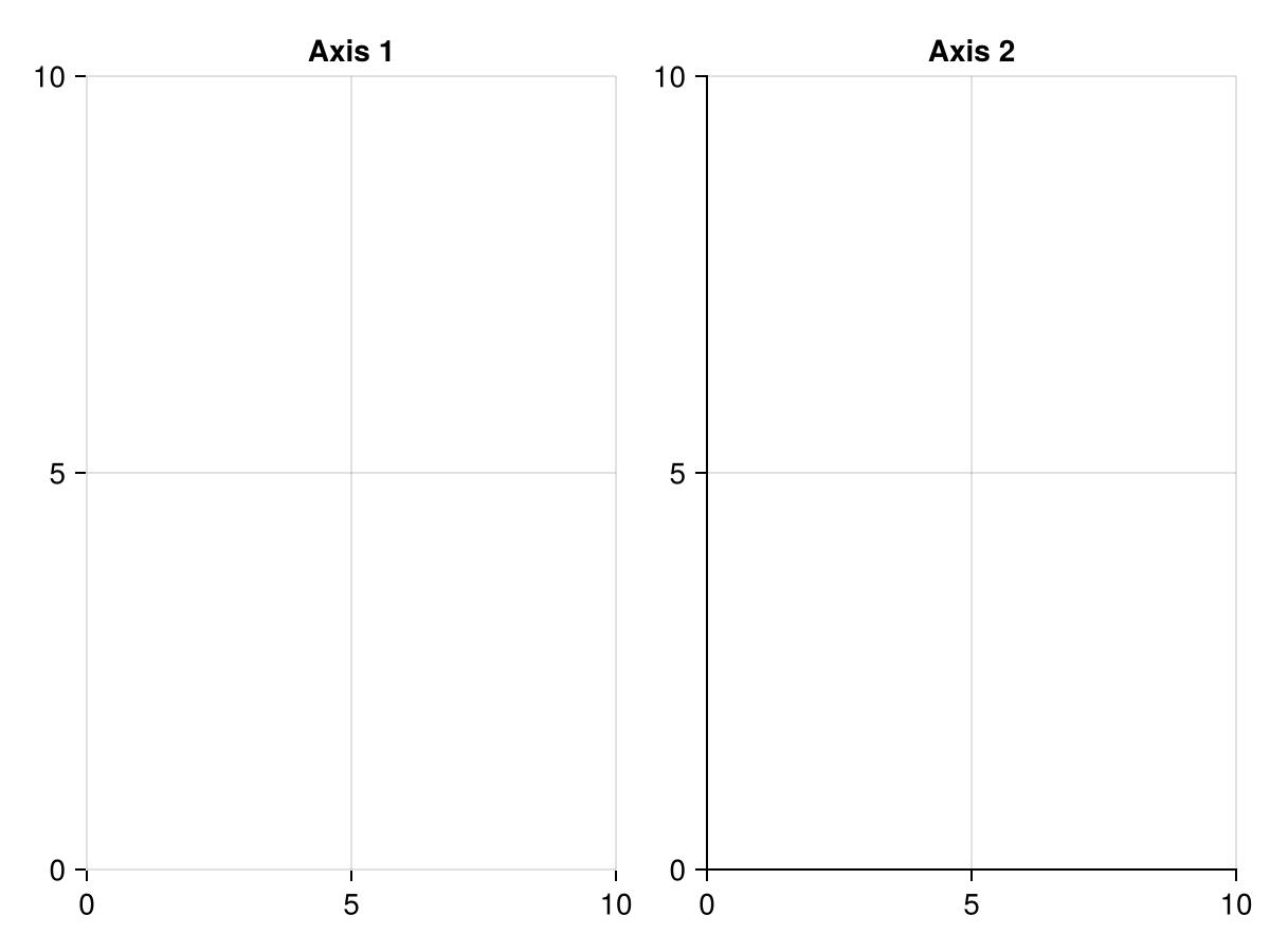
Makie自带图像布局的网格管理, 构建fig=Figure()以后, 可以通过fig[row,col]的语法来指定绘制子图的布局:

julia

x = LinRange(0, 10, 100)
y = sin.(x)

fig = Figure()
lines(fig[1, 1], x, y, color = :red)
lines(fig[1, 2], x, y, color = :blue)
lines(fig[2, 1:2], x, y, color = :green)

fig

julia

还可以先创建空的Axis, 然后再绘制:

julia

fig = Figure()
ax1 = Axis(fig[1, 1])
ax2 = Axis(fig[1, 2])
ax3 = Axis(fig[2, 1:2])
fig

lines!(ax1, 0..10, sin)
lines!(ax2, 0..10, cos)
lines!(ax3, 0..10, sqrt)
fig

julia

图例

Makie中可以用Legend()函数来手动添加图例, 该函数接受绘图对象作为参数:

julia

fig = Figure()
ax1, l1 = lines(fig[1, 1], 0..10, sin, color = :red)
ax2, l2 = lines(fig[2, 1], 0..10, cos, color = :blue)
Legend(fig[1:2, 2], [l1, l2], ["sin", "cos"])
fig

julia

Colorbar()也是一种图列, 适用于Heatmap()等颜色变化的图

julia

fig, ax, hm = heatmap(randn(20, 20))
Colorbar(fig[1, 2], hm)
fig

julia

布局教程

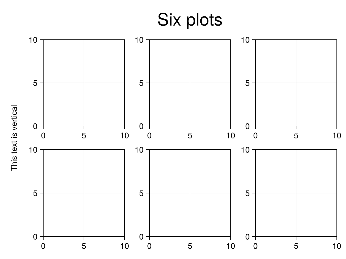
Makie可以进行非常细致的布局控制, 比如以下图例:

对应的代码:

julia

using CairoMakie
using Makie.FileIO

f = Figure(backgroundcolor = RGBf(0.98, 0.98, 0.98),
    resolution = (1000, 700))
ga = f[1, 1] = GridLayout()
gb = f[2, 1] = GridLayout()
gcd = f[1:2, 2] = GridLayout()
gc = gcd[1, 1] = GridLayout()
gd = gcd[2, 1] = GridLayout()

# deal with grid A:
axtop = Axis(ga[1, 1])
axmain = Axis(ga[2, 1], xlabel = "before", ylabel = "after")
axright = Axis(ga[2, 2])
# align plots
linkyaxes!(axmain, axright)
linkxaxes!(axmain, axtop)

labels = ["treatment", "placebo", "control"]
data = randn(3, 100, 2) .+ [1, 3, 5]

for (label, col) in zip(labels, eachslice(data, dims = 1))
    scatter!(axmain, col, label = label)
    density!(axtop, col[:, 1])
    density!(axright, col[:, 2], direction = :y)
end

# 设置图形紧贴坐标轴
ylims!(axtop, low = 0)
xlims!(axright, low = 0)

# 设置坐标轴breaks和label
axmain.xticks = 0:3:9
axtop.xticks = 0:3:9

# 添加图例
leg = Legend(ga[1, 2], axmain)

# 隐藏附图的内容, 对齐图和图例
hidedecorations!(axtop, grid = false)
hidedecorations!(axright, grid = false)
leg.tellheight = true

# 控制图间距
colgap!(ga, 10)
rowgap!(ga, 10)

# 添加标题
Label(ga[1, 1:2, Top()], "Stimulus ratings", valign = :bottom,
    font = :bold,
    padding = (0, 0, 5, 0))

# GridLayout B:

xs = LinRange(0.5, 6, 50)
ys = LinRange(0.5, 6, 50)
data1 = [sin(x^1.5) * cos(y^0.5) for x in xs, y in ys] .+ 0.1 .* randn.()
data2 = [sin(x^0.8) * cos(y^1.5) for x in xs, y in ys] .+ 0.1 .* randn.()

ax1, hm = contourf(gb[1, 1], xs, ys, data1,
    levels = 6)
ax1.title = "Histological analysis"
contour!(ax1, xs, ys, data1, levels = 5, color = :black)
hidexdecorations!(ax1)

ax2, hm2 = contourf(gb[2, 1], xs, ys, data2,
    levels = 6)
contour!(ax2, xs, ys, data2, levels = 5, color = :black)
# 添加colorbar
cb = Colorbar(gb[1:2, 2], hm, label = "cell group")
# 设置colorbar上下界
low, high = extrema(data1)
edges = range(low, high, length = 7)
centers = (edges[1:6] .+ edges[2:7]) .* 0.5
cb.ticks = (centers, string.(1:6))
# 对齐
cb.alignmode = Mixed(right = 0)
# 间距
colgap!(gb, 10)
rowgap!(gb, 10)


# GridLayout C:
brain = load(assetpath("brain.stl"))

ax3d = Axis3(gc[1, 1], title = "Brain activation")
m = mesh!(
    ax3d,
    brain,
    color = [tri[1][2] for tri in brain for i in 1:3],
    colormap = Reverse(:magma),
)
Colorbar(gc[1, 2], m, label = "BOLD level")

# GridLayout D:
axs = [Axis(gd[row, col]) for row in 1:3, col in 1:2]
hidedecorations!.(axs, grid = false, label = false)

for row in 1:3, col in 1:2
    xrange = col == 1 ? (0:0.1:6pi) : (0:0.1:10pi)

    eeg = [sum(sin(pi * rand() + k * x) / k for k in 1:10)
        for x in xrange] .+ 0.1 .* randn.()

    lines!(axs[row, col], eeg, color = (:black, 0.5))
end

axs[3, 1].xlabel = "Day 1"
axs[3, 2].xlabel = "Day 2"

Label(gd[1, :, Top()], "EEG traces", valign = :bottom,
    font = :bold,
    padding = (0, 0, 5, 0))

rowgap!(gd, 10)
colgap!(gd, 10)

for (i, label) in enumerate(["sleep", "awake", "test"])
    Box(gd[i, 3], color = :gray90)
    Label(gd[i, 3], label, rotation = pi/2, tellheight = false)
end

colgap!(gd, 2, 0)

n_day_1 = length(0:0.1:6pi)
n_day_2 = length(0:0.1:10pi)

colsize!(gd, 1, Auto(n_day_1))
colsize!(gd, 2, Auto(n_day_2))

# 添加ABCD标签
for (label, layout) in zip(["A", "B", "C", "D"], [ga, gb, gc, gd])
    Label(layout[1, 1, TopLeft()], label,
        fontsize = 26,
        font = :bold,
        padding = (0, 5, 5, 0),
        halign = :right)
end

colsize!(f.layout, 1, Auto(0.5))

rowsize!(gcd, 1, Auto(1.5))

f

julia

长宽比和尺寸控制

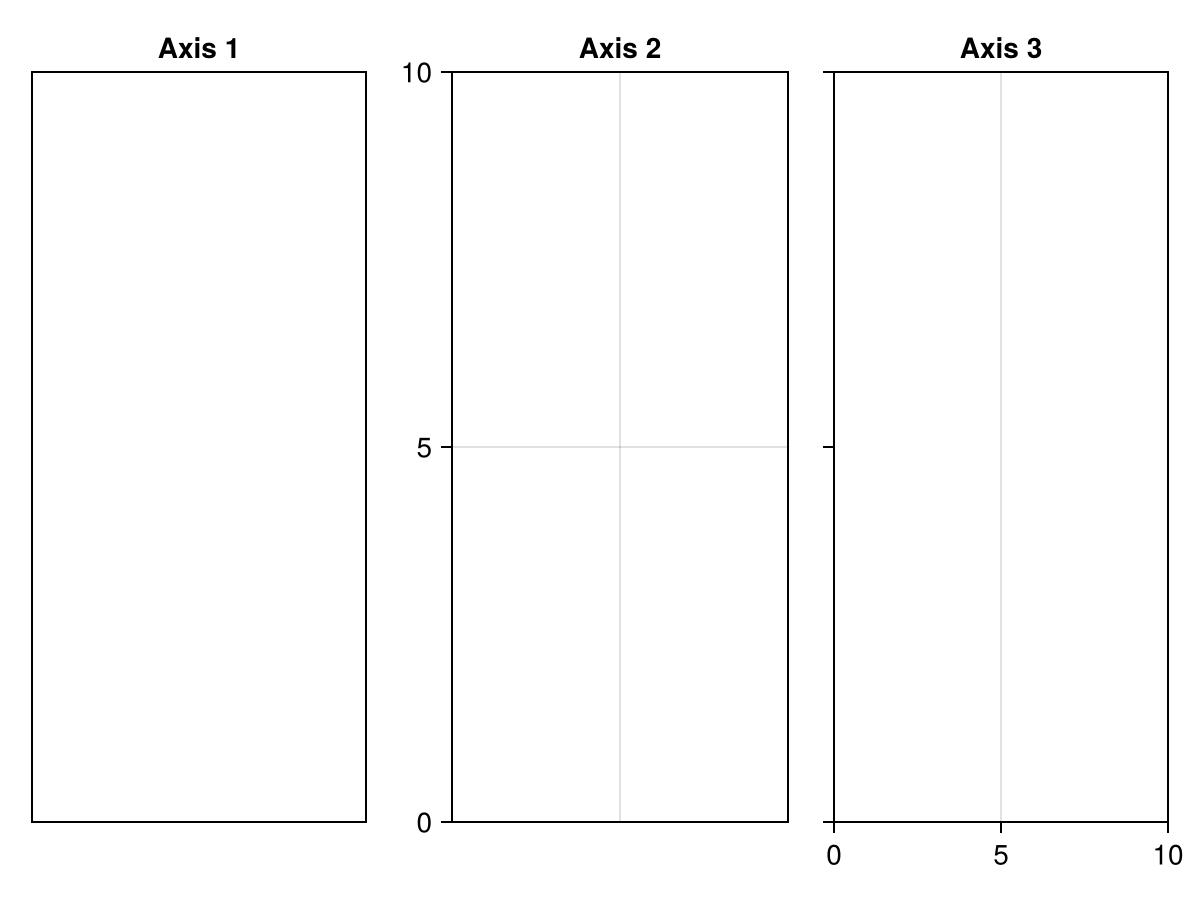
控制长宽比和尺寸是绘图中的常见需求, 比如许多图需要正方形的axes, Axis有一个aspect属性来控制长宽比:

julia

set_theme!(backgroundColor = :gray90)

f = Figure(resolution = (800, 500))
ax = Axis(f[1, 1], aspect = 1)
Colorbar(f[1,2])
f

julia

可以发现一个问题, 方形的axis和colorbar之间间距很大, 这是为什么呢?

通过向axis所在单元格添加一个Box来看看:

julia

Box(f[1, 1], color = (:red, 0.2), strokewidth = 0)
f

julia

可以看到aspect的实际作用是减少了Axis的尺寸, 而布局没有做相应的适配改变。 因此, 大多数时候, 我们应该直接操作布局, 而不是Axis的长宽比。

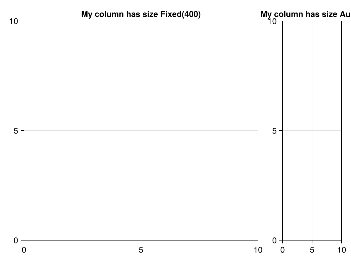
GridLayout()默认的宽和高是Auto(), 就是根据内容自动适应. 如果想要固定宽高, 则需要把内容设置为Aspect:

julia

ax = Axis(f[1, 1])
Colorbar(f[1, 2])
colsize!(f.layout, 1, Aspect(1, 1.0))
f

julia

此时图就正常了:

还可以用colsize!()函数更改Grid的长宽比:

julia

ax.aspect = 0.5 # 手动更改aspect
f # 轴和colorbar又拉大间距了

colsize!(f.layout, 1, Aspect(1, 0.5)) # 再设定Grid的长款比
f # 又ok了

julia

还有一个resize_to_layout!()函数, 将图形大小调整为布局所有内容所需要的大小, 这样Grid上下左右的留白也会尽可能的少: resize_to_layout!(f); f

绘图概念解释

Backends

  • GLMakie: GPU支持的, 独立窗口绘制2D和3D图形, 可以实现交互绘图;

  • CairoMakie: 基于Cairo.jl的非交互式绘图, 用于绘制出版矢量图;

  • WGLMakie: 基于WebGL, 浏览器中运行的3D和3D交互绘图;

  • RPRMakie: 光线追踪后端(实验性质, 一般不用)

Backends基础操作
julia

# 激活
using CairoMakie
CairoMakie.activate!()
##  XXX.activate!()函数可以接收一些关键字参数, 如:
using GLMakie
GLMakie.activate!(title="My title", fxaa = false)

julia

具体的关键字参数, 见上表超链接中每个Backend的详细文档, 内容有点多, 就不一一列举了。

Figures

Makie中一个完整的绘图用Figure对象表示, 一般包含一个顶层的Scene和一个GridLayout, 以及放入其中的各种Blocks:

  • Figure

    • Scene

    • GridLayout

      • Blocks

Figures基本属性
  • 创建: 可以通过f = Figure(...)或者非叹号绘图函数, 如fig, ax, p = scatter(rand(100,2))

  • 添加Blocks: Blocks将其父Figure当作第一个参数, 可以通过索引语法进行添加: ax = f[1, 1] = Axis(f);

  • GridPositionGridSubposition控制Grid位置f[1, 2];

  • figure_padding控制padding;

  • contents()content()返回指定GridPosition的对象:

julia

f = Figure()
box = f[1:3, 1:2] = Box(f)
ax = f[1, 1] = Axis(f)

contents(f[1, 1]) == [ax]
contents(f[1:3, 1:2]) == [box, ax]
contents(f[1:3, 1:2], exact = true) == [box]

# 如果一个位置只有一个对象, 用content(), 这样返回的是一个对象, 而不是像contents()一样返回一个Vector, 如果不能确定只有一个对象, content()会报错
f = Figure()
ax = f[1, 1] = Axis(f)

contents(f[1, 1]) == [ax]
content(f[1, 1]) == ax

julia

  • size = (width, height)控制尺寸, 此后其他的单位数值都是相对的了, 如size=(600, 400);linewidth=10可以预期为线宽是整个图像的1/60;

  • px_per_unitpt_per_unit分别控制位图和矢量图的尺寸, 如px_per_unit = 1表示尺寸数值1表示一个像素, 则上述size=(600, 400)会输出600x400像素的图;pt是一个适用于矢量图的印刷单位, 定义为1/72英寸, 或0.353毫米, CairoMakie默认的大小为: px_per_unit = 0.75, px_per_unit = 2

Scenes

Cameras

Camera定义一个Scene的视角(投射), 在Makie中, 甚至可以把2D图投射到3D(WOW!)

目前支持通过camera关键字传递以下Camera构造方法:

  • campixel!: Pixel Camera => 将场景投射到像素空间中(将数据的整数步长映射到一个像素点), 无control;

  • cam_relative!: Relative Camera => 将场景投射到0.1 x 0.1的空间中, 无control;

  • cam2d!: 2D Camera => 使用具有固定旋转和纵行比的正投影(orthographic projection), 有以下关键字参数:

    • zoomspeed = 0.10f0: 鼠标滚轮缩放速度;

    • zoombutton = nothing: 添加缩放按钮;

    • panbutton = Mouse.right: 设置平移视图的按钮;

    • selectionbutton = (Keyboard.space, Mouse.left): 设置控制矩形选框缩放的按钮;

Note 该Camera不能用于Axis, 默认用于LSceneScene
  • Camera3D

  • cam3d!

  • cam3d_cad!

Warn 3D Camera参数众多, 这里不过多介绍, 详情见: HERE

GridLayouts

Makie通过GridLayout对Scene中的元素进行布局设定, 布局通常包含以下属性:

  • 建议边界

  • 计算边界

  • 自动确定高宽

  • Protrusions(突出部分? 4个角的控制:(l,r,t,b))

  • 尺寸属性

  • 对齐属性

具体见Layouts

Blocks

  • Blocks是可以添加到Figure或Scene的对象, 其位置和大小由GridLayout控制

  • Block有其自己内部的Gridlayout

  • 可以通过设置bbox参数来将Block放置到指定位置:

BBox(l, r, b, t)函数通过控制边界创建一个Rect2f

julia

using CairoMakie
f = Figure()
Axis(f, bbox = BBox(100, 300, 100, 500), title="Axis 1")
Axis(f, bbox = BBox(400, 700, 200, 400), title="Axis 2")

julia
  • 可以通过delete!(block)函数删除block

Makie支持的blocks有:

  • Axis, Axis3, PolarAxis

  • GridLayout

  • LScene

  • Box

  • 交互: Button, IntervalSlider, Menu, Slider, SliderGrid, Toggle

  • 标注: Colorbar, Legend, Label, Textbox

Colors

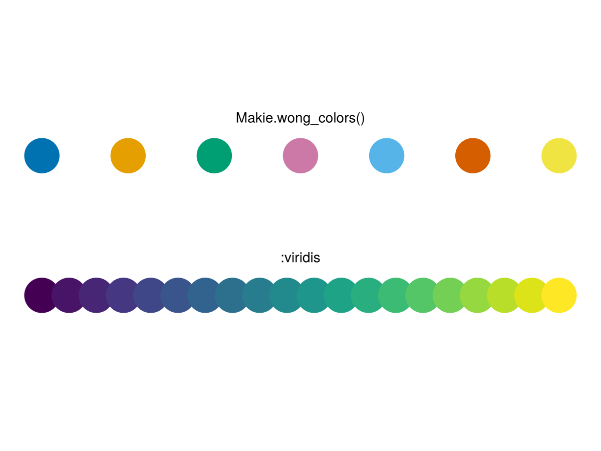
  • 大多数绘图对象支持传递color属性, 元素要与元素数目保持一致(或单个颜色, 广播到所有元素);

  • 当传递数字数组(或单个数字时), 用colormapcolorrange属性将其转换成颜色值

    • colormap: 连续映射;

    • colorrange: 离散映射;

    • NaN值默认为:transparent颜色, 可以通过nan_color属性更改

    • 超过映射范围的颜色, 默认用极值颜色, 可以通过lowcliphighclip属性更改

  • Makie中没有alpha/opacity等显式声明透明度的关键字, 可以用(color, alpha)元组来设置透明度

具名颜色

Makie通过Colors.jl来解析具名颜色(使用CSS规范), 可以在 这里找到所有具名颜色信息。

调色板

  • Makie默认离散调色板是Makie.wong_colors()

  • Makie默认连续调色板是:viridis

  • 可以在ColorSchemes.jl中查找调色板信息

Note 这里 查看所有Makie支持的预设调色板

Fonts

Makie用FreeType.jl包来控制字体, 具体内容略

  • 目前Makie不支持绘制表情符号(emoji);

  • 目前不支持彩色字体

Headless

原文在此

Makie可以用在无显示器的系统中:

  • CairoMakie正常使用;

  • 通过设置X11转发(ssh -X user@host)实现GLMakie的使用;

  • 通过JSServe控制监听端口实现WGLMakie的使用;

Theming

Makie支持通过属性更改绘图主题的几乎每个细节, 这主要通过以下三个函数实现:

  • set_theme!

  • update_theme!

  • with_theme

`set_theme!`
set_theme!(theme; kwargs ...)

  • 不带参数调用, 重置为默认;

  • kwargs可以是各种支持的属性关键字;

julia

using CarioMakie

function example_plot()
    f = Figure()
    for i in 1:2, j in 1:2
        lines(f[i, j], cumsum(randn(50)))
    end
    Label(f[0, :], "A simple example plot")
    Label(f[3, :], L"Random walks $x(t_n)$")
    f
end

example_plot()

julia
julia

fontsize_theme = Theme(fontsize = 10)
set_theme!(fontsize_theme)
example_plot()

julia

merge Makie的主题通常只影响部分属性, 所以允许通过merge()将多个主题组合应用:

julia

dark_latexfonts = merge(theme_dark(), theme_latexfonts())
with_theme(dark_latexfonts) do
    example_plot()
end

julia

`update_theme!` 可以使用update_theme!(attr...)部分更新已经激活的主题
julia

update_theme!(fontsize=30)
example_plot()

julia
`with_theme` with_theme(theme, attr...) do plot end with_theme(plot, theme)

julia

lines_theme = Theme(
    Lines = (
        linewidth = 4,
        linestyle = :dash,
    )
)

with_theme(example_plot, lines_theme)

ggplot_theme = Theme(
    Axis = (
        backgroundcolor = :gray90,
        leftspinevisible = false,
        rightspinevisible = false,
        bottomspinevisible = false,
        topspinevisible = false,
        xgridcolor = :white,
        ygridcolor = :white,
    )
)
with_theme(example_plot, ggplot_theme)

julia
`Cycles` Makie的主题支持绘图属性的周期性循环设置, 循环规则必须作为绘图对象的属性给出:

julia

with_theme(
    Theme(
        palette = (color = [:red, :blue], marker = [:circle, :xcross]),
        Scatter = (cycle = [:color, :marker],) # <== 设置按照颜色和形状循环, 总共有2x2=4组
    )) do
    scatter(fill(1, 10))  # <== 第1组[:color, :marker]
    scatter!(fill(2, 10)) # <== 第2组[:color, :marker]
    scatter!(fill(3, 10)) # <== 第3组[:color, :marker]
    scatter!(fill(4, 10)) # <== 第4组[:color, :marker]
    scatter!(fill(5, 10)) # <== 第1组[:color, :marker]
    current_figure()
end

julia

还可以通过Cycle()构造函数定义一个Cycle对象, 允许设置covary关键字, 会将所有covary=true的循环器的所有属性循环在一起(可以理解成zip?):

julia

with_theme(
    Theme(
        palette = (color = [:red, :blue], linestyle = [:dash, :dot]),
        Lines = (cycle = Cycle([:color, :linestyle], covary = true),) # 这里只有两套循环了,而不是四套
    )) do
    lines(fill(5, 10))
    lines!(fill(4, 10))
    lines!(fill(3, 10))
    lines!(fill(2, 10))
    lines!(fill(1, 10))
    current_figure()
end

julia

还可以通过Cycled对象手动配置当前应该应用哪一套主题循环, Cycled对象记录主题循环的迭代器, 可以通过索引i来指定访问某一套:

julia

using CairoMakie

f = Figure()

Axis(f[1, 1])

# the normal cycle
lines!(0..10, x -> sin(x) - 1)
lines!(0..10, x -> sin(x) - 2)
lines!(0..10, x -> sin(x) - 3)

# manually specified colors
lines!(0..10, x -> sin(x) - 5, color = Cycled(3))
lines!(0..10, x -> sin(x) - 6, color = Cycled(2))
lines!(0..10, x -> sin(x) - 7, color = Cycled(1))

f

julia

Cycle会在Palettes中查找指定属性, 可以通过配置palettepatchcolor来控制:

julia

using CairoMakie

f = Figure(size = (800, 800))
# 默认调色板
Axis(f[1, 1], title = "Default cycle palette")
for i in 1:6
    density!(randn(50) .+ 2i)
end

# 手动设置调色板
Axis(f[2, 1],
    title = "Custom cycle palette",
    palette = (patchcolor = [:red, :green, :blue, :yellow, :orange, :pink],))

for i in 1:6
    density!(randn(50) .+ 2i)
end

# 清空调色板
set_theme!(Density = (cycle = [],))
Axis(f[3, 1], title = "No cycle")

for i in 1:6
    density!(randn(50) .+ 2i)
end

f

julia

misc theme还可以通过rowgapcolgap更改默认网格布局间隔。

预设主题

  • default: 这个个人觉得就很好看

  • theme_ggplot2: ggplot2主题

  • theme_minimal: 这个比较适合我, 最简洁

  • theme_black: 黑色主题

  • theme_light: 黑色主题的白色版

  • theme_dark: 黑色主题的灰色版

Inspecting Data

交互式数据检查器, 可以鼠标悬停展示数据信息, 应该只能在GLMakie中使用,暂略。

原文在此

LaTeX

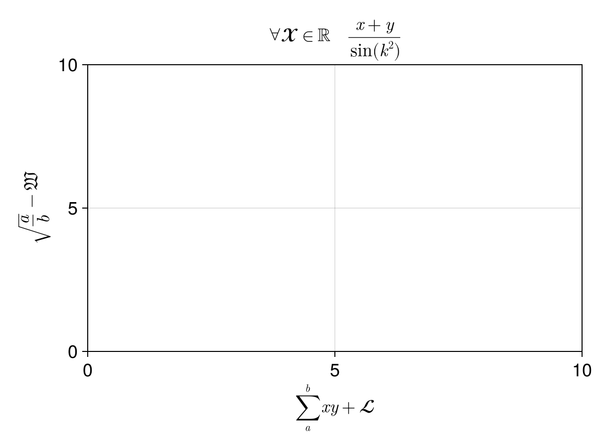
Makie通过LaTeXStrings.jl和MathTeXEngine.jl包提供LaTeX的支持, 可以在输入文本的时候输入LaTeX格式的公式, LaTeXString对象可以用L""字符串宏创建:
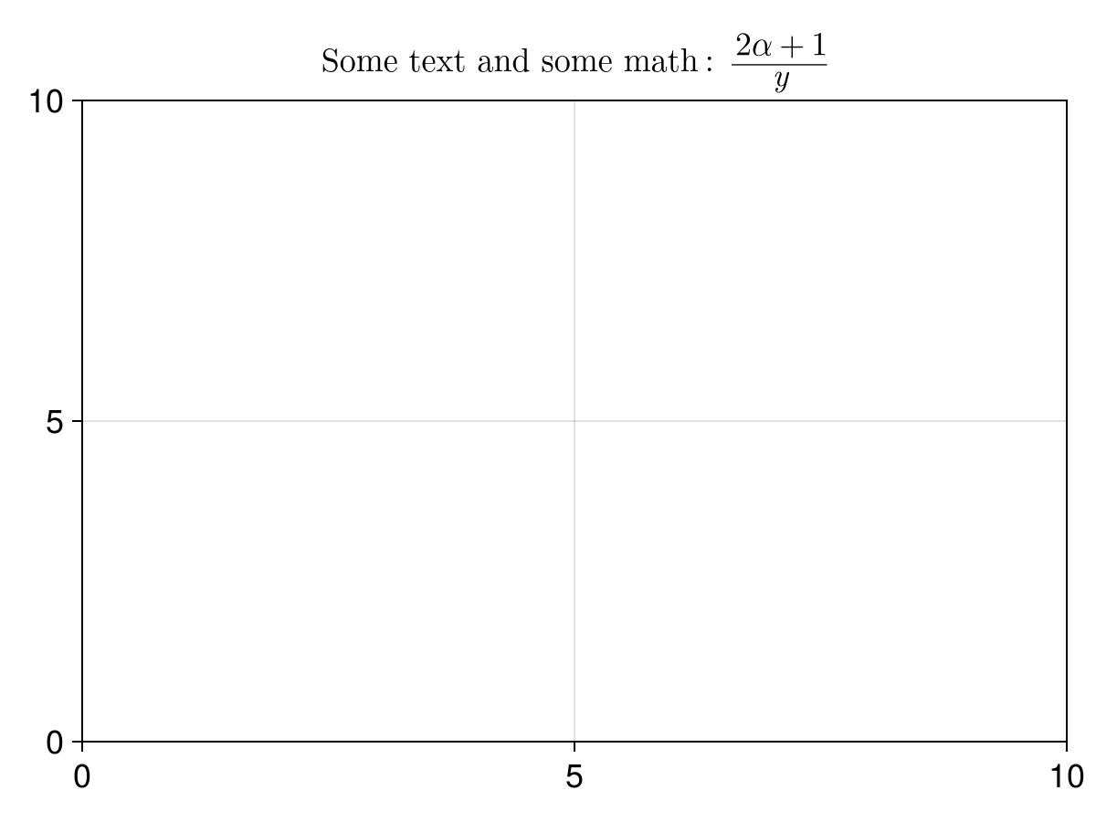
julia

using CairoMakie

f = Figure(fontsize = 18)

Axis(f[1, 1],
    title = L"\forall \mathcal{X} \in \mathbb{R} \quad \frac{x + y}{\sin(k^2)}",
    xlabel = L"\sum_a^b{xy} + \mathscr{L}",
    ylabel = L"\sqrt{\frac{a}{b}} - \mathfrak{W}"
)

f

julia

甚至可以混用文本和数学公式:

julia

using CairoMakie

f = Figure(fontsize = 18)
t = "text"
Axis(f[1,1], title=L"Some %$(t) and some math: $\frac{2\alpha+1}{y}$")

f

julia

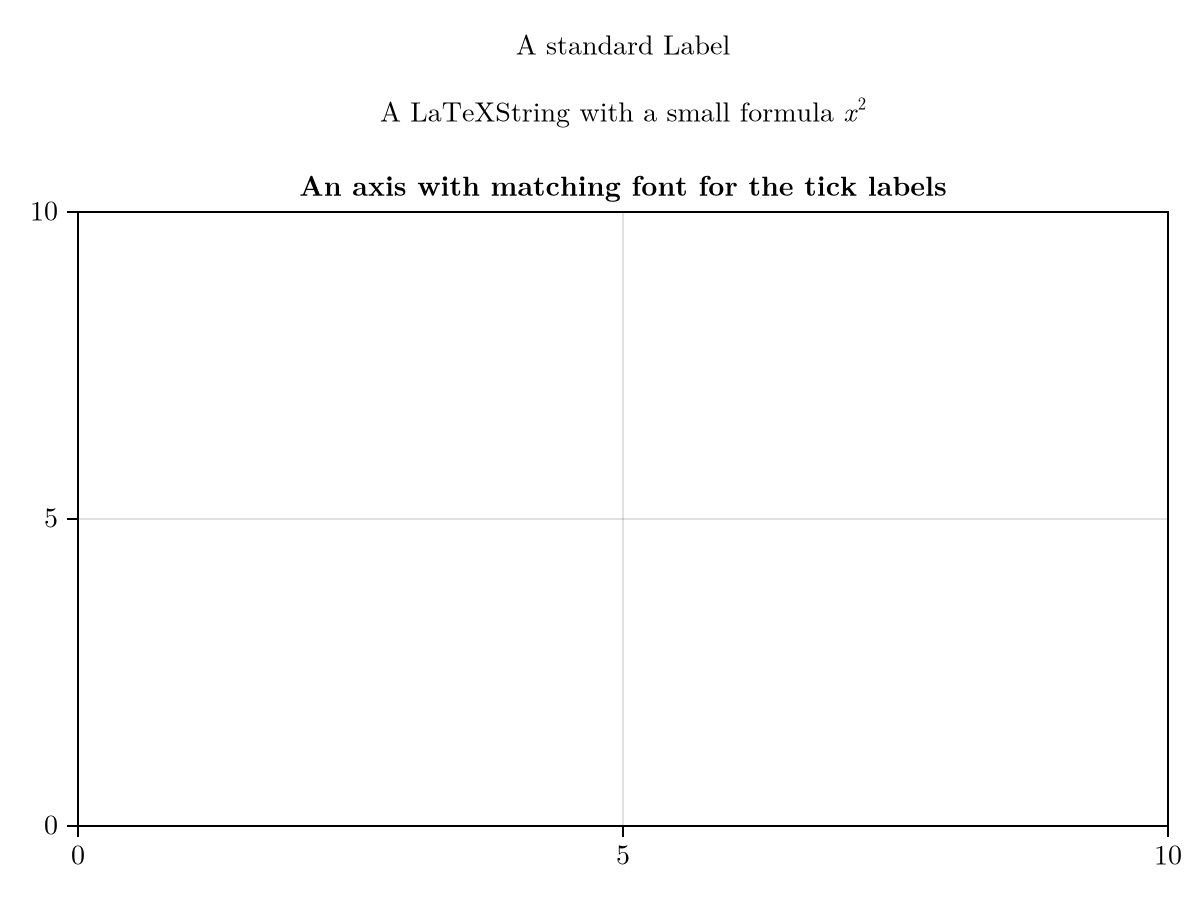
Makie提供了一个theme_latexfonts()主题, 自动支持latex:

julia

using CairoMakie

with_theme(theme_latexfonts()) do
    fig = Figure()
    Label(fig[1, 1], "A standard Label", tellwidth = false)
    Label(fig[2, 1], L"A LaTeXString with a small formula $x^2$", tellwidth = false)
    Axis(fig[3, 1], title = "An axis with matching font for the tick labels")
    fig
end

julia

SpecApi

Basic transparency

Observables and Interaction

Makie提供了一个方法可以动态检测数据的改变, 实时更新图片, 从而能够绘制动画, 实现这些用的就是 observables.jl

  • Observable是一个容器对象, 允许交互地更新值;

  • 每个Observable对象都有一个类型参数, 规定存储值的类型;

julia

using GLMakie, Makie
x = Observable(0.0)
x2 = Observable{Real}(0.0)
x3 = Observable{Any}(0.0)

julia
  • 可以用x[]空索引的形式来更新Observable对象: x[] = 3.34

  • 可以用on(x) do ... end语法来定义对象更新后自动执行的操作:

julia

on(x) do x
    println("new value of x is $x")
end

x[] = 5.0

# new value of x is 5.0

julia

Note 如果使用in-place语法(如 x .= colorant"red" )更新Observable, 则需要用notify(x)显式地触发on的动作
Info Observable中所有注册函数会按照注册顺序同步执行, 所以连续更改两个Observable, 会先把第一个更改的所有函数执行后, 再更新第二个
  • Observable值的访问有两种方法:

    • to_value函数: value = to_value(x), 用to_value的好处是, 也可以对非Observable变量使用(此时返回变量原始值), 保持代码格式统一;

    • 空索引: value = x[], 所以x[] = x[]这种语法, 就是用老的x值更新x, 等于不改变x,但是又触发了一次更新操作, 似乎等于notify(x)?;

  • 连接多个observable: lift

lift(function, Observable), 用来创建新的Observable, 其值的更新依赖于另一个Observable:
julia

f(x) = x^2

y = lift(f, x) # 更新x会同步更新y

z = lift(y) do y
    -y
end

x[] = 10.0
@show x[] #10.0
@show y[] # 100.0
@show z[] # -100.0

y[] = 20 # 更改y, z会随着更新, 但x不会

julia

当有众多变量需要联动的时候, 写lift函数有点麻烦, Makie还提供了一个@lift宏, 用来方便地简化该操作: z = @lift($x .+ $y)

  • 宏中需要在变量前加上$;

  • 也支持多行语句:

julia

multiline_node = @lift begin
    a = $x[1:50] .* $y[51:100]
    b = sum($z)
    a .- b
end

julia
  • 支持访问表达式或复杂结构的子元素:

julia

container = (x = Observable(1), y = Observable(2))
@lift($(container.x) + $(container.y))

julia
  • 多重触发同步更新问题

Warn 实际应用中, 会有很多基于多个Observable的方法, 但由于Observable的特性, 只能一一更改变量, 如果一个函数依赖于两个没有建立lift的Observable, 就会多次触发, 比如:
julia

xs = Observable(1:10)
ys = Observable(rand(10))

zs = @lift($xs .+ $ys) # xs和ys是两个独立的Observable

# 现在更新xs和ys
xs[] = 2:11 # 此时触发了一次zs
ys[] = rand(10) # 此时又触发了一次zs

julia
上述例子中, 似乎只是效率的问题, 但实际上这还可能会引起错误: 比如如果我是push!更改了xs的长度, 此时ys的长度没变, 触发的zs更新动作就会报错。

有一种方法可以只更新数值, 但不触发更新操作xs.val:

julia

xs.val = 1:11 # 更新了xs, 但不触发监听器
ys[] = rand(11) # 更新y后再触发监听, 此时更新zs

julia

这种操作还是尽量避免用, 因为代码有可能会因此变得复杂, 最好的方法就是合理设计Observable的联动, 把复杂的依赖用自定义类型的方式组合更新, 避免出现这种情况。

Animations

通过record()函数记录Observables的改动, 可以创建动画:

julia

using GLMakie
using Makie.Colors

fig, ax, lineplot = lines(0..10, sin; linewidth=10)

# animation settings
nframes = 30
framerate = 30
hue_iterator = range(0, 360, length=nframes)

record(fig, "color_animation.mp4", hue_iterator;
        frametrate = framerate) do hue
    lineplot.color = HSV(hue, 1, 0.75)
end

# 或者可以用 record(function, fig, "file", ...)的语法:
function change_function(hue)
    lineplot.color = HSV(hue, 1, 0.75)
end

record(change_function, fig, "color_animation.mp4", hue_iterator; framerate = framerate)

julia
  • 支持的文件格式: .mkv, .mp4, .webm, .gif

Events

Makie用Events结构存储Observables的改变, 并用events(x)访问, Events包含如下字段:

  • window_area::Observable{Rect2i}: 当前视窗大小(像素)

  • window_dpi::Observable{Float64}: 视窗DPI

  • window_open::Observable{Bool}: 视窗是否打开

  • hasfocus::Observable{Bool}: 窗口是否被聚焦(在前台)

  • entered_window::Observable{Bool}: 鼠标是否在窗口内(悬停, 无论是否聚焦)

  • mousebutton::Observable{MouseButtonEvent}

  • mousebuttonstate::Set{Mouse.Button}

  • mouseposition::Observable{NTuple{2, Float64}}

  • scroll::Observable{NTuple{2, Float64}}

  • keyboardbutton::Observable{KeyEvent}

  • keyboardstate::Observable{Keyboard.Button}: 当前按下的所有键

  • unicode_input::Observable{Char}: 最近输入的字符

  • dropped_files::Observable{Vector{String}}: 拖拽加载的文件路径

Warn Events中包含丰富的交互配置项, 这里不展开了:

Plot Recipes

Makie可以让用户通过Recipes自定义自己的画图函数。主要有两种Recipe:

  • Type recipes: 本质上就是类型转换, 规定用户自定义类型到现有绘图类型的映射关系;

  • Full recipes: 自定义新的绘图函数, 更底层。

Type Recipes

Makie中类型的转换顺序如下

  1. 先尝试通过convert_arguments(::PlotType, args...)进行派发;

  2. 如果没有找到匹配的方法, 则再尝试通过conversion_trait(::PlotType)确定转换特征

  3. 尝试通过convert_arguments(::ConversionTrait, args...)分派;

  4. 尝试用convert_signle_arguments递归地转换每一个参数;

  5. 尝试用convert_arguments(::PlotType, converted_args...)分派;

  6. Failed

多参数转换: convert_arguments 例如, 定义一个新的Circle绘图类型, 可以解析成Point向量: convert_arguments(x::Circle) = (decompose(Point2f, x),)

convert_arguments必须始终返回Tuple
  • 可以用类型子集来定义转换, 如各种散点图:

convert_arguments(P::Type{<:Scatter}, x::MyType) = convert_arguments(P, rand(10, 10))
  • 预设一些转换特征, 可以方便地定义一组共享相同特征的绘图类型的行为:

    • NoConversion

    • PointBased

    • SurfaceLike

    • VolumeLike

  • 可以多个参数一起转换:

    • convert_arguments(P::Type{<:Scatter}, x::MyType, y::MyOtherType) = ...

  • 可以将转换设置成默认绘图类型:

    • plottype(::MyType) = Surface

单参数转换: convert_single_argument convert_single_argument可以用来把Makie未知类型转换成其他类型。
Todo 这一部分文档好晦涩啊, 没有示例!

使用@recipe的完整配方(Full Recipe)

Full Recipe包含两个部分:

  • 绘图类型名称MyPlot, 和@recipe定义的参数和主题信息

  • 至少一个plot!定义的绘图方法, 使用其他现有绘图函数进行实现

第一部分: @recipe

举个栗子:

julia

@recipe(MyPlot, x, y, z) do scene
    Theme(
        plot_color = :red
    )
end

julia

以上@recipe宏实际上会被展开成如下操作:

  • 类型定义: const MyPlot{ArgTypes} = Combined{myplot, ArgTypes}, 定义一个从大骆驼名称(类型)到小写名称(方法)的映射关系;

  • 自动定义myplot(args...)myplot!(args...)方法;

  • 如果提供了参数列表(x, y, z), 则会发出argument_names的声明:

    • argument_names(::Type{<:MyPlot}) = (:x, :y, :z)

    • 这样就可以用诸如plot_object[:x]的语法来获取第一个参数;

    • 或者, 永远可以用plot_object[i]来获取第i个参数;

  • @recipe中设定的主题参数插入到绘制MyPlot的任何场景默认主题中;

第二部分: plot!方法

plot!来定义MyPlot的具体绘图方案, 如:

julia

function plot!(myplot::MyPlot)
    # normal plotting code, building on any previously defined recipes
    # or atomic plotting operations, and adding to the combined `myplot`:
    lines!(myplot, rand(10), color = myplot[:plot_color])
    plot!(myplot, myplot[:x], myplot[:y])
    myplot
end

julia
具体案例: 股票开盘/收盘可视化 假设我们想用开盘/收盘高/低的分类来可视化股票(我们自定义一个类型来保存信息), 下面我们来定义配方:

  • 首先创建一个存股票的数据结构:

julia

struct StockValue{T<:Real}
    open::T
    close::T
    high::T
    low::T
end

julia
  • 然后创建一个StockChart绘图类型, 其中do scene闭包只是一个返回默认属性的函数, 将下跌和上涨的股票分别标记成greenred:

julia

@recipe(StockChart) do scene
    Attributes(
        downcolor = :red,
        upcolor = :green,
    )
end

julia
  • 然后创建绘图方法:

julia

function Makie.plot!(sc::StockChart{>:Tuple{AbstractVector{<:Real}, AbstractVector{<:StockValue}}})
    times = sc[1] 
    stockvalues = sc[2] # (open, close, high, low)

    # 定义画图元素: 
    linesegs = Observable(Point2f[])
    bar_froms = Observable(Float32[])
    bar_tos = Observable(Float32[])
    colors = Observable(Bool[])

    # 定义一个更新函数, 当输入参数有变化时, 更新图内容
    function update_plot(times, stockvalues)
        colors[]
        # 清空之前内容
        empty!(linesegs[])
        empty!(bar_froms[])
        empty!(bar_tos[])
        empty!(colors[])

        # 用更新的值重新填充
        for (t, s) in zip(times, stockvalues)
            push!(linesegs[], Point2f(t, s.low))
            push!(linesegs[], Point2f(t, s.high))
            push!(bar_froms[], s.open)
            push!(bar_tos[], s.close)
        end
        append!(colors[], [x.close > x.open for x in stockvalues])
        colors[] = colors[] # Observable变量的用法
    end

    # 检测到数值变化的时候就启动更新函数
    Makie.Observables.onany(update_plot, times, stockvalues)
    update_plot(times[], stockvalues[])

    # 定义颜色, 我们的例子是分类变量:
    colormap = Observable{Any}()
    map!(colormap, sc.downcolor, sc.upcolor) do dc, uc
        [dc, uc]
    end

    # 画图
    linesegments!(sc, linesegs, color = colors, colormap = colormap)
    barplot!(sc, times, bar_froms, fillto = bar_tos, color = colors, strokewidth = 0, colormap = colormap)

    # 返回图形
    sc # ?? 这个sc跟输入的sc是同一个? 
end

julia

测试一下:

julia

timestamps = 1:100

# we create some fake stock values in a way that looks pleasing later
startvalue = StockValue(0.0, 0.0, 0.0, 0.0)
stockvalues = foldl(timestamps[2:end], init = [startvalue]) do values, t
    open = last(values).close + 0.3 * randn()
    close = open + randn()
    high = max(open, close) + rand()
    low = min(open, close) - rand()
    push!(values, StockValue(
        open, close, high, low
    ))
end

# now we can use our new recipe
f = Figure()

stockchart(f[1, 1], timestamps, stockvalues)

# and let's try one where we change our default attributes
stockchart(f[2, 1], timestamps, stockvalues,
    downcolor = :purple, upcolor = :orange)
f

julia

动态输入逐帧更新
julia

timestamps = Observable(collect(1:100))
stocknode = Observable(stockvalues)

fig, ax, sc = stockchart(timestamps, stocknode)

record(fig, "stockchart_animation.mp4", 101:200,
        framerate = 30) do t
    # push a new timestamp without triggering the observable
    push!(timestamps[], t)

    # push a new StockValue without triggering the observable
    old = last(stocknode[])
    open = old.close + 0.3 * randn()
    close = open + randn()
    high = max(open, close) + rand()
    low = min(open, close) - rand()
    new = StockValue(open, close, high, low)
    push!(stocknode[], new)

    # now both timestamps and stocknode are synchronized
    # again and we can trigger one of them by assigning it to itself
    # to update the whole stockcharts plot for the new frame
    stocknode[] = stocknode[]
    # let's also update the axis limits because the plot will grow
    # to the right
    autolimits!(ax)
end

julia

绘图参考

Blocks

Axis

Axis的属性

  • alignmode: Axis相对与其父GridLayout的对齐模式, 默认是Inside()

  • aspect: 长宽比, 默认为nothing

    • noting

    • DataAspect(): 按照数据自动适配长宽比

    • AxisAspect(ratio): 自定义

  • autolimitaspect: 可选nothing或数字, 默认是nothing, 如果设置为数字, 则自动调整aspect的比例(类似于PS中锁定长宽比)

  • backgroundcolor: 默认:white

  • bottom/left/top/rightspinecolor: 默认:black

  • bottom/left/top/rightspinevisible: true

  • flip_ylabel: 是否反转ylabel, false

  • h/valign: 水平/垂直对齐方式, :center

  • height/width: 高宽, nothing

  • limits: (noting, noting), 可以是(xlow, xhigh, ylow, yhigh)四元元组, 也可以用xlims!()ylims!()limits!()来快捷设置

  • panbutton: 交互选项, 平移按钮

  • spinewidth: 轴宽, 默认1.0

  • [sub]title: 默认"", 可以是text基本绘图支持的对象, 比如数学公式

  • [sub]titlecolor: 默认@inherit :textcolor :black

  • [sub]titlefont: 默认:regular

  • [sub]titlegap: 默认0

  • [sub]titlelineheight: 默认1

  • [sub]titlesize: 默认@inherit :fontsize 16.0f0

  • [sub]titlevisible: true

  • titlealign: :center

  • tellheight/width: true, 高宽是否能被父Layout控制

  • x/yautolimitmargin: 默认(0.05f0, 0.05f0)

  • x/yaxisposition: 默认:bottom(x)和:left(y), 可选: x: [:bottom, :top], y: [:left, :right]

  • x/ygridcolor: x/y内部网格线颜色, 默认RGBAf(0, 0, 0, 0.12)

  • x/ygridstyle: 网格线类型, 默认nothing

  • x/ygridvisible: 默认true

  • x/ygridwidth: 默认1.0

  • x/ylabel: ""

  • x/ylabelcolor: @inherit :textcolor :black

  • x/ylabelfont: :regular

  • x/ylabelpadding: 3.0

  • x/ylabelrotation: Makie.automatic, 可以是弧度值, 如pi/2

  • x/ylabelsize: @inherit :fontsize 16.0f0

  • x/ylabelvisible: true

  • x/yminorgridcolor: RGBAf(0, 0, 0, 0.05)

  • x/yminorgridvisible: true

  • x/yminorgirdwidth: 1.0

  • x/yminortickalign: 0.0

  • x/yminortickcolor: :black

  • x/yminorticks: IntervalsBetween(2)或者数字向量, 定义刻度间隔

  • x/yminorticksize: 4.0

  • x/yminorticksvisible: false

  • x/yminortickwidth: 1.0

  • x/ypankey/lock: 交互的绑定

  • x/yrectzoom: true, 交互缩放是否影响尺寸

  • x/yreversed: false, 坐标轴反向

  • x/yscale: identity, 坐标轴缩放投射函数, 可以是任何可逆函数, 一些预定义选项:

  • identity, log, log2, log10, sqrt, logit, Makie.pseudolog10, Makie.Symlog10

  • x/ytickalgin

  • x/ytickcolor

  • x/ytickformat

  • x/yticklabelalign

  • x/yticklabelcolor

  • x/yticklabelfont

  • x/yticklabelpad

  • x/yticklabelrotation

  • x/yticklabelsize

  • x/yticks

  • x/yticksize

  • x/yticksmirrored: 是否在对侧也显示刻度线

  • x/yticksvisible

  • x/ytickswidth

  • x/ytrimspine: false, 是否将轴的范围限制到最外侧主刻度线(就是控制x和y是否会在0点交汇)

  • x/yzoomkey, x/yzoomlock

默认Axis是2D布局, 有以下操作:

  • 定义: ax = Axis(f[1,1], xlabel="x", ylabel="y", title="Title")

  • 绘图(2d图形): lineobj = lines!(ax, 0..10, sin, color=:red)

  • 删除和清空: delete!(ax, plotobj); empty!(ax)

julia

using CairoMakie


f = Figure()

axs = [Axis(f[1, i]) for i in 1:3]

scatters = map(axs) do ax
    [scatter!(ax, 0:0.1:10, x -> sin(x) + i) for i in 1:3]
end

delete!(axs[2], scatters[2][2])
empty!(axs[3])

f

julia
  • 隐藏边框和提示: hidespines!(), hidedecorations!()

julia

using CairoMakie


f = Figure()

ax1 = Axis(f[1, 1], title = "Axis 1")
ax2 = Axis(f[1, 2], title = "Axis 2")

hidespines!(ax1)
hidespines!(ax2, :t, :r) # only top and right

f

julia

julia

using CairoMakie


f = Figure()

ax1 = Axis(f[1, 1], title = "Axis 1")
ax2 = Axis(f[1, 2], title = "Axis 2")
ax3 = Axis(f[1, 3], title = "Axis 3")

hidedecorations!(ax1)
hidexdecorations!(ax2, grid = false)
hideydecorations!(ax3, ticks = false)

f

julia

  • 对齐:

    • linkyaxes!()linkxaxes!(): 对齐Axes

    • xticklabelspace()yticklabelspace(): 控制坐标轴标题和轴的距离, 保证标题对齐

  • 创建双坐标轴: 目前没有专门的函数, 可以添加新坐标轴(设置yaxisposition), 然后隐藏新轴的内容:

julia

using CairoMakie

f = Figure()

ax1 = Axis(f[1, 1], yticklabelcolor = :blue)
ax2 = Axis(f[1, 1], yticklabelcolor = :red, yaxisposition = :right)
hidespines!(ax2)
hidexdecorations!(ax2)

lines!(ax1, 0..10, sin, color = :blue)
lines!(ax2, 0..10, x -> 100 * cos(x), color = :red)

f

julia
  • 交互操作: 在GLMakie等可以交互的后端中, 可以进行如下交互式操作:

    • 鼠标滚动缩放

    • 拖拽平移

    • Ctrl + leftclick重置

    • 选框缩放

    • 还可以用register_interaction!()deregister_interaction!()函数自定义交互

    • interactions(ax)检查当前可用的交互

    • activate_interaction!()deactivate_interaction!()激活和停用交互

    • 自定义交互函数: 暂略, 用时再补充

Axis3

三维坐标系, 平时不常用, 先略过, 详情见 Makie-Ref-Axis3

Box

可以设置圆角的矩形块, 不是基本的画图元素, 而是在Axis之外的设备, 所以个人感觉平时不怎么常用, 可以用来做顶层的高亮, 或者占位, 或者用来研究Layout的布局。

常用参数:

Box(fig[1,1], args...)
  • color

  • cornerradius: 圆角半径, 一个数字或四个数字(右上角顺时针: RT, RB, LB, LT)

  • 其他通用参数略

Button

这个更不常用了, 交互的时候才用得上的, 略过, 原文: Button

Colorbar

一种Legend, 默认参数会自动识别载入图像的阈值进行绘制:

julia

xs = LinRange(0, 20, 50)
ys = LinRange(0, 15, 50)
zs = [cos(x) * sin(y) for x in xs, y in ys]
fig = Figure()
ax, hm = heatmap(fig[1, 1][1, 1], xs, ys, zs)
Colorbar(fig[1,1][1,2], hm)
fig

julia

也可以手动指定:

julia

fig = Figure()
Axis(fig[1,1])
Colorbar(fig[1,2], limits = (0, 10), colormap = :viridis,flipaxis = false)
fig

julia
常用属性

  • colormap: @inherit :colormap :viridis

  • colorrange: nothing

  • label...: label, labelcolor, labelfont, labelpadding, labelrotation, labelsize, labelvisible

  • limits: nothing, 颜色条的范围

  • low/highclip: nothing, 上下界三角号

  • nsteps: 100, 颜色梯度

  • scale: identity, 颜色刻度

  • size: 16, 高度或宽度(取决于是竖直还是水平), 可以被width/height覆盖

  • 其他通用参数略

GridLayout

设置长宽的主要途径, 目前有四种模式:

  • Fixed(scene_units): 固定大小, 通常不常用:

julia

f = Figure()
Axis(f[1, 1], title = "My column has size Fixed(400)")
Axis(f[1, 2], title = "My column has size Auto()")
colsize!(f.layout, 1, Fixed(400))
f

julia
  • Relative(fraction): 锁定长宽缩放比:

julia

f = Figure()

Axis(f[1, 1], title = "My column has size Relative(2/3)")
Axis(f[1, 2], title = "My column has size Auto()")
Colorbar(f[1, 3])
colsize!(f.layout, 1, Relative(2/3))
f

julia

  • Auto() == Auto(true, 1): 自动适应

  • Aspect(reference, ratio): 设置Grid Cell的长宽比, 而不改变Layout的比例(前文已说过)

Grids是可以嵌套的, 具体的略, 见前文

常用属性/方法

  • trim!(f.layout): 删除fig中未使用的空间

  • colgap!(), rowgap!(): 调整行列的间距, colgap!(f.lyaout, 1, Relative(0.15))

IntervalSlider

略, 交互图的时候用的, 虽然很炫酷, 但平时基本用不到

原文 HERE

Label

Label就是位于矩形边框中的文本, 与text不同之处在于, 其halignvalign属性始终是针对未旋转的状态(可以理解为对矩形边框设置h和valign, 而不是对文本)

julia

using CairoMakie

fig = Figure()

fig[1:2, 1:3] = [Axis(fig) for _ in 1:6]

supertitle = Label(fig[0, :], "Six plots", fontsize = 30)

sideinfo = Label(fig[2:3, 0], "This text is vertical", rotation = pi/2)

fig

julia
属性

  • alignmode: Inside()

  • color

  • font, fontsize

  • h/valign

  • width, height

  • justification: :center, 文本对齐方式: (:left, :right, :center)

  • lineheight, padding, rotation

  • text

  • visible

  • word_wrap: false, 文本是否自动换行

Legend

  • 图列可以通过传递图列条目向量, 标签向量以及可选标题等参数进行构建。

  • 图列条目向量可以是:

    • 绘图对象

    • LegendElement: LineElement, MarkerElement, PolyElement

Legend element attributes

  • 基本绘图模块通常预定义了绘图元素到图例元素的转换, 如Scatter => MarkerElement; Lines => LineElement;

  • 图例默认值继承主题

julia

using CairoMakie
f = Figure()
Axis(f[1, 1])
xs = 0:0.5:10
ys = sin.(xs)
lin = lines!(xs, ys, color = :blue)
sca = scatter!(xs, ys, color = :red)
sca2 = scatter!(xs, ys .+ 0.5, color = 1:length(xs), marker = :rect)
Legend(f[1, 2],
    [lin, sca, [lin, sca], sca2],
    ["a line", "some dots", "both together", "rect markers"])
f

julia
从Axis创建图例 可以把Axis对象(如Axis, LSence, Scene等)传递给Legend()进行创建, 默认会按照绘图的图层顺序排列图例:

julia

f = Figure()
ax = f[1, 1] = Axis(f)
lines!(0..15, sin, label = "sin", color = :blue)
lines!(0..15, cos, label = "cos", color = :red)
lines!(0..15, x -> -cos(x), label = "-cos", color = :green)
f[1, 2] = Legend(f, ax, "Trig Functions", framevisible = false)
f

julia

可以用mergeunique关键字处理有相同标签的绘图对象:

  • merge=true: 合并绘图元素到一个legend元素;

  • unique=true: 按照[标签, 绘图类型]两个标准进行去重;

julia

f = Figure()
traces = cumsum(randn(10, 5), dims = 1)
for (i, (merge, unique)) in enumerate(
        Iterators.product([false, true], [false true]))
    axis = Axis(f[fldmod1(i, 2)...],
        title = "merge = $merge, unique = $unique")
    for trace in eachcol(traces)
        lines!(trace, label = "single", color = (:black, 0.2))
    end
    mu = vec(sum(traces, dims = 2) ./ 5)
    lines!(mu, label = "mean")
    scatter!(mu, label = "mean")
    axislegend(axis, merge = merge, unique = unique)
end
f

julia
Multi-Bank Legend 在图列元素很多的时候, 可以使用nbanks属性控制单行元素数目。vertical mode下, Bank是列, horizontal下是行:
julia

using CairoMakie
f = Figure()
Axis(f[1, 1])
xs = 0:0.1:10
lins = [lines!(xs, sin.(xs .+ 3v), color = RGBf(v, 0, 1-v)) for v in 0:0.1:1]
Legend(f[1, 2], lins, string.(1:length(lins)), nbanks = 3)
f

julia
Lengend in Axis 可以用axislegend把图列嵌入到图像Axis中, 通过设置position,h/valign属性调节位置, 提供预设的关键字配置:[lrc][btc]:
julia

# halign
l => left
r => right
c => center
# valign
b => bottom
t => top
c => center
:lb #左下

julia

一个例子:

julia

using CairoMakie
f = Figure()
ax = Axis(f[1, 1])
sc1 = scatter!(randn(10, 2), color = :red, label = "Red Dots")
sc2 = scatter!(randn(10, 2), color = :blue, label = "Blue Dots")
scatter!(randn(10, 2), color = :orange, label = "Orange Dots")
scatter!(randn(10, 2), color = :cyan, label = "Cyan Dots")
axislegend() # 默认位于右上
axislegend("Titled Legend", position = :lb) # 可以只传入标题
axislegend(ax, [sc1, sc2], ["One", "Two"], "Selected Dots", position = :rb,
    orientation = :horizontal) # 也可以跟legend函数一样手动配置
f

julia

除了用axislegend之外, 也可以用Legend手动设置成在axis内画图, 需要:

  • 把legend和axis画到同一个layout;

  • 配置legend的tellheighttellwidthfalse;

  • 控制margin关键字防止边界重叠;

例如:

julia

using CairoMakie
haligns = [:left, :right, :center]
valigns = [:top, :bottom, :center]
f = Figure()
Axis(f[1, 1])
xs = 0:0.1:10
lins = [lines!(xs, sin.(xs .* i), color = color)
    for (i, color) in zip(1:3, [:red, :blue, :green])]
for (j, ha, va) in zip(1:3, haligns, valigns)
    Legend(
        f[1, 1], lins, ["Line $i" for i in 1:3],
        "$ha & $va",
        tellheight = false,
        tellwidth = false,
        margin = (10, 10, 10, 10),
        halign = ha, valign = va, orientation = :horizontal
    )
end
f

julia

手动创建Legend 可以使用LineElement, MarkerElement, PolyElement来DIY图例:

# 直接构造元素时, 可以省略`[]`中的部分

# LineElement
[line]points, [line]color, linestyle, linewidth

# MarkerElement
[marker]points, marker, markersize, [marker]color,
[marker]strokewidth, [marker]strokecolor

# PolyElement
[poly]points, [poly]color, [poly]strokewidth, [poly]strokecolor

利用Point()基础集合元素来定义形状。Point()有一些变体: Point(), Point2f(), Point3(), Point3f(), Point4(), Point4f()。 Legend中的元素绘图区, 会限制在[(0, 0), (1, 1)]的区间内, 所以通常用Point2f()[0, 1]范围内绘图(实际上也可以超过这个范围, 但是图会很丑)

julia

using CairoMakie
f = Figure()
Axis(f[1, 1])
elem_1 = [LineElement(color = :red, linestyle = nothing),
          MarkerElement(color = :blue, marker = 'x', markersize = 15,
          strokecolor = :black)]
elem_2 = [PolyElement(color = :red, strokecolor = :blue, strokewidth = 1),
          LineElement(color = :black, linestyle = :dash)]
elem_3 = LineElement(color = :green, linestyle = nothing,
        points = Point2f[(0, 0), (0, 1), (1, 0), (1, 1)])
elem_4 = MarkerElement(color = :blue, marker = 'π', markersize = 15,
        points = Point2f[(0.2, 0.2), (0.5, 0.8), (0.8, 0.2)])
elem_5 = PolyElement(color = :green, strokecolor = :black, strokewidth = 2,
        points = Point2f[(0, 0), (1, 0), (0, 1)])
Legend(f[1, 2],
    [elem_1, elem_2, elem_3, elem_4, elem_5],
    ["Line & Marker", "Poly & Line", "Line", "Marker", "Poly"],
    patchsize = (35, 35), rowgap = 10)
f

julia

多组图例 当有多个图例分组的时候, 可以存成一个Legend向量, 然后批量操作, 配合titleposition, nbanks等属性控制:

julia

using CairoMakie

f = Figure()

markersizes = [5, 10, 15, 20]
colors = [:red, :green, :blue, :orange]

group_size = [MarkerElement(marker = :circle, color = :black,
    strokecolor = :transparent,
    markersize = ms) for ms in markersizes]

group_color = [PolyElement(color = color, strokecolor = :transparent)
    for color in colors]

legends = [Legend(f,
    [group_size, group_color],
    [string.(markersizes), string.(colors)],
    ["Size", "Color"], tellheight = true) for _ in 1:4]

f[1, 1:2] = legends[1:2]
f[2, :] = legends[3]
f[3, :] = legends[4]

for l in legends[3:4]
    l.orientation = :horizontal
    l.tellheight = true
    l.tellwidth = false
end

legends[2].titleposition = :left
legends[4].titleposition = :left

legends[1].nbanks = 2
legends[4].nbanks = 2

Label(f[1, 1, Left()], "titleposition = :top\norientation = :vertical\nnbanks = 2", font = :italic, padding = (0, 10, 0, 0))
Label(f[1, 2, Right()], "titleposition = :left\norientation = :vertical\nnbanks = 1", font = :italic, padding = (10, 0, 0, 0))
Label(f[2, 1:2, Top()], "titleposition = :top, orientation = :horizontal\nnbanks = 1", font = :italic)
Label(f[3, 1:2, Top()], "titleposition = :left, orientation = :horizontal\nnbanks = 2", font = :italic)

f

julia

Legend的具体关键字参数略。

LSene

暂时用不到, 暂略。

交互配置, 暂时用不到, 暂略。

PolarAxis

Warn PolarAxis目前是Makie中的实验功能, 其语法和功能可能会有改动。而且需要在v"0.19"以上版本才能使用。

定义极坐标系用PolarAxis方法, 跟Axis用法类似:

julia

using CairoMakie
f = Figure()
ax = PolarAxis(f[1, 1], title = "Title")
f

julia

绘图语法与Axis类似, 区别是需要定义thetar:radian(角度和半径), 而不是x, y

julia

f = Figure(resolution = (800, 400))

ax = PolarAxis(f[1, 1], title = "Theta as x")
lineobject = lines!(ax, 0..2pi, sin, color = :red)

ax = PolarAxis(f[1, 2], title = "R as x", theta_as_x = false)
scatobject = scatter!(range(0, 10, length=100), cos, color = :orange)

f

julia

可以控制rlimitsthetalimits, 从而绘制扇形图和局部圆环图:

julia

f = Figure(resolution = (600, 600))

ax = PolarAxis(f[1, 1], title = "Default")
lines!(ax, range(0, 8pi, length=300), range(0, 10, length=300))
ax = PolarAxis(f[1, 2], title = "thetalimits", thetalimits = (-pi/6, pi/6))
lines!(ax, range(0, 8pi, length=300), range(0, 10, length=300))

ax = PolarAxis(f[2, 1], title = "rlimits", rlimits = (5, 10))
lines!(ax, range(0, 8pi, length=300), range(0, 10, length=300))
ax = PolarAxis(f[2, 2], title = "both")
lines!(ax, range(0, 8pi, length=300), range(0, 10, length=300))
thetalims!(ax, -pi/6, pi/6)
rlims!(ax, 5, 10)

f

julia

还可以通过theta_0direction来控制旋转:

julia

f = Figure()

ax = PolarAxis(f[1, 1], title = "Reoriented Axis", theta_0 = -pi/2, direction = -1)
lines!(ax, range(0, 8pi, length=300), range(0, 10, length=300))
thetalims!(ax, -pi/6, pi/6)
rlims!(ax, 5, 10)

f

julia
Polar兼容的绘图类型

  • line, scatter;

  • heatmap: 部分兼容, 在CairoMakie上可用, 在GLMakie上不行, 可以用voronoiplot替代;

  • surface: image的替品

  • image: 不兼容

julia

f = Figure(resolution = (800, 500))

ax = PolarAxis(f[1, 1], title = "Surface")
rs = 0:10
phis = range(0, 2pi, 37)
cs = [r+cos(4phi) for phi in phis, r in rs]
p = surface!(ax, 0..2pi, 0..10, cs, shading = false, colormap = :coolwarm)
ax.gridz[] = 100
tightlimits!(ax) # surface plots include padding by default
Colorbar(f[2, 1], p, vertical = false, flipaxis = false)

ax = PolarAxis(f[1, 2], title = "Voronoi")
rs = 1:10
phis = range(0, 2pi, 37)[1:36]
cs = [r+cos(4phi) for phi in phis, r in rs]
p = voronoiplot!(ax, phis, rs, cs, show_generators = false, strokewidth = 0)
rlims!(ax, 0.0, 10.5)
Colorbar(f[2, 2], p, vertical = false, flipaxis = false)

f

julia

其他交互的block

Slider, SliderGrid, Textbox, Toggle

Plots

太长不全翻了, 只挑一些关键的信息记录 原文在此: Blocks; Plots

<<<<<<< HEAD

Scene

Howtos

Observables

Makie提供了一个方法可以动态检测数据的改变, 实时更新图片, 从而能够绘制动画, 实现这些用的就是 observables.jl

  • Observable是一个容器对象, 允许交互地更新值;

  • 每个Observable对象都有一个类型参数, 规定存储值的类型;

julia

using GLMakie, Makie
x = Observable(0.0)
x2 = Observable{Real}(0.0)
x3 = Observable{Any}(0.0)

julia
  • 可以用x[]空索引的形式来更新Observable对象: x[] = 3.34

  • 可以用on(x) do ... end语法来定义对象更新后自动执行的操作:

julia

on(x) do x
    println("new value of x is $x")
end

x[] = 5.0

# new value of x is 5.0

julia

Note 如果使用in-place语法(如 x .= colorant"red" )更新Observable, 则需要用notify(x)显式地触发on的动作
Info Observable中所有注册函数会按照注册顺序同步执行, 所以连续更改两个Observable, 会先把第一个更改的所有函数执行后, 再更新第二个
  • Observable值的访问有两种方法:

    • to_value函数: value = to_value(x), 用to_value的好处是, 也可以对非Observable变量使用(此时返回变量原始值), 保持代码格式统一;

    • 空索引: value = x[], 所以x[] = x[]这种语法, 就是用老的x值更新x, 等于不改变x,但是又触发了一次更新操作, 似乎等于notify(x)?;

  • 连接多个observable: lift

lift(function, Observable), 用来创建新的Observable, 其值的更新依赖于另一个Observable:
julia

f(x) = x^2

y = lift(f, x) # 更新x会同步更新y

z = lift(y) do y
    -y
end

x[] = 10.0
@show x[] #10.0
@show y[] # 100.0
@show z[] # -100.0

y[] = 20 # 更改y, z会随着更新, 但x不会

julia

当有众多变量需要联动的时候, 写lift函数有点麻烦, Makie还提供了一个@lift宏, 用来方便地简化该操作: z = @lift($x .+ $y)

  • 宏中需要在变量前加上$;

  • 也支持多行语句:

julia

multiline_node = @lift begin
    a = $x[1:50] .* $y[51:100]
    b = sum($z)
    a .- b
end

julia
  • 支持访问表达式或复杂结构的子元素:

julia

container = (x = Observable(1), y = Observable(2))
@lift($(container.x) + $(container.y))

julia
  • 多重触发同步更新问题

Warn 实际应用中, 会有很多基于多个Observable的方法, 但由于Observable的特性, 只能一一更改变量, 如果一个函数依赖于两个没有建立lift的Observable, 就会多次触发, 比如:
julia

xs = Observable(1:10)
ys = Observable(rand(10))

zs = @lift($xs .+ $ys) # xs和ys是两个独立的Observable

# 现在更新xs和ys
xs[] = 2:11 # 此时触发了一次zs
ys[] = rand(10) # 此时又触发了一次zs

julia
上述例子中, 似乎只是效率的问题, 但实际上这还可能会引起错误: 比如如果我是push!更改了xs的长度, 此时ys的长度没变, 触发的zs更新动作就会报错。

有一种方法可以只更新数值, 但不触发更新操作xs.val:

julia

xs.val = 1:11 # 更新了xs, 但不触发监听器
ys[] = rand(11) # 更新y后再触发监听, 此时更新zs

julia

这种操作还是尽量避免用, 因为代码有可能会因此变得复杂, 最好的方法就是合理设计Observable的联动, 把复杂的依赖用自定义类型的方式组合更新, 避免出现这种情况。

Recipes

Makie可以让用户通过Recipes自定义自己的画图函数。主要有两种Recipe:

  • Type recipes: 本质上就是类型转换, 规定用户自定义类型到现有绘图类型的映射关系;

  • Full recipes: 自定义新的绘图函数, 更底层。

Type Recipes

Makie中类型的转换顺序如下

  1. 先尝试通过convert_arguments(::PlotType, args...)进行派发;

  2. 如果没有找到匹配的方法, 则再尝试通过conversion_trait(::PlotType)确定转换特征

  3. 尝试通过convert_arguments(::ConversionTrait, args...)分派;

  4. 尝试用convert_signle_arguments递归地转换每一个参数;

  5. 尝试用convert_arguments(::PlotType, converted_args...)分派;

  6. Failed

多参数转换: convert_arguments 例如, 定义一个新的Circle绘图类型, 可以解析成Point向量: convert_arguments(x::Circle) = (decompose(Point2f, x),)

convert_arguments必须始终返回Tuple
  • 可以用类型子集来定义转换, 如各种散点图:

convert_arguments(P::Type{<:Scatter}, x::MyType) = convert_arguments(P, rand(10, 10))
  • 预设一些转换特征, 可以方便地定义一组共享相同特征的绘图类型的行为:

    • NoConversion

    • PointBased

    • SurfaceLike

    • VolumeLike

  • 可以多个参数一起转换:

    • convert_arguments(P::Type{<:Scatter}, x::MyType, y::MyOtherType) = ...

  • 可以将转换设置成默认绘图类型:

    • plottype(::MyType) = Surface

单参数转换: convert_single_argument convert_single_argument可以用来把Makie未知类型转换成其他类型。
Todo 这一部分文档好晦涩啊, 没有示例!

使用@recipe的完整配方(Full Recipe)

Full Recipe包含两个部分:

  • 绘图类型名称MyPlot, 和@recipe定义的参数和主题信息

  • 至少一个plot!定义的绘图方法, 使用其他现有绘图函数进行实现

第一部分: @recipe

举个栗子:

julia

@recipe(MyPlot, x, y, z) do scene
    Theme(
        plot_color = :red
    )
end

julia

以上@recipe宏实际上会被展开成如下操作:

  • 类型定义: const MyPlot{ArgTypes} = Combined{myplot, ArgTypes}, 定义一个从大骆驼名称(类型)到小写名称(方法)的映射关系;

  • 自动定义myplot(args...)myplot!(args...)方法;

  • 如果提供了参数列表(x, y, z), 则会发出argument_names的声明:

    • argument_names(::Type{<:MyPlot}) = (:x, :y, :z)

    • 这样就可以用诸如plot_object[:x]的语法来获取第一个参数;

    • 或者, 永远可以用plot_object[i]来获取第i个参数;

  • @recipe中设定的主题参数插入到绘制MyPlot的任何场景默认主题中;

第二部分: plot!方法

plot!来定义MyPlot的具体绘图方案, 如:

julia

function plot!(myplot::MyPlot)
    # normal plotting code, building on any previously defined recipes
    # or atomic plotting operations, and adding to the combined `myplot`:
    lines!(myplot, rand(10), color = myplot[:plot_color])
    plot!(myplot, myplot[:x], myplot[:y])
    myplot
end

julia
具体案例: 股票开盘/收盘可视化 假设我们想用开盘/收盘高/低的分类来可视化股票(我们自定义一个类型来保存信息), 下面我们来定义配方:

  • 首先创建一个存股票的数据结构:

julia

struct StockValue{T<:Real}
    open::T
    close::T
    high::T
    low::T
end

julia
  • 然后创建一个StockChart绘图类型, 其中do scene闭包只是一个返回默认属性的函数, 将下跌和上涨的股票分别标记成greenred:

julia

@recipe(StockChart) do scene
    Attributes(
        downcolor = :red,
        upcolor = :green,
    )
end

julia
  • 然后创建绘图方法:

julia

function Makie.plot!(sc::StockChart{>:Tuple{AbstractVector{<:Real}, AbstractVector{<:StockValue}}})
    times = sc[1] 
    stockvalues = sc[2] # (open, close, high, low)

    # 定义画图元素: 
    linesegs = Observable(Point2f[])
    bar_froms = Observable(Float32[])
    bar_tos = Observable(Float32[])
    colors = Observable(Bool[])

    # 定义一个更新函数, 当输入参数有变化时, 更新图内容
    function update_plot(times, stockvalues)
        colors[]
        # 清空之前内容
        empty!(linesegs[])
        empty!(bar_froms[])
        empty!(bar_tos[])
        empty!(colors[])

        # 用更新的值重新填充
        for (t, s) in zip(times, stockvalues)
            push!(linesegs[], Point2f(t, s.low))
            push!(linesegs[], Point2f(t, s.high))
            push!(bar_froms[], s.open)
            push!(bar_tos[], s.close)
        end
        append!(colors[], [x.close > x.open for x in stockvalues])
        colors[] = colors[] # Observable变量的用法
    end

    # 检测到数值变化的时候就启动更新函数
    Makie.Observables.onany(update_plot, times, stockvalues)
    update_plot(times[], stockvalues[])

    # 定义颜色, 我们的例子是分类变量:
    colormap = Observable{Any}()
    map!(colormap, sc.downcolor, sc.upcolor) do dc, uc
        [dc, uc]
    end

    # 画图
    linesegments!(sc, linesegs, color = colors, colormap = colormap)
    barplot!(sc, times, bar_froms, fillto = bar_tos, color = colors, strokewidth = 0, colormap = colormap)

    # 返回图形
    sc # ?? 这个sc跟输入的sc是同一个? 
end

julia

测试一下:

julia

timestamps = 1:100

# we create some fake stock values in a way that looks pleasing later
startvalue = StockValue(0.0, 0.0, 0.0, 0.0)
stockvalues = foldl(timestamps[2:end], init = [startvalue]) do values, t
    open = last(values).close + 0.3 * randn()
    close = open + randn()
    high = max(open, close) + rand()
    low = min(open, close) - rand()
    push!(values, StockValue(
        open, close, high, low
    ))
end

# now we can use our new recipe
f = Figure()

stockchart(f[1, 1], timestamps, stockvalues)

# and let's try one where we change our default attributes
stockchart(f[2, 1], timestamps, stockvalues,
    downcolor = :purple, upcolor = :orange)
f

julia

动态输入逐帧更新
julia

timestamps = Observable(collect(1:100))
stocknode = Observable(stockvalues)

fig, ax, sc = stockchart(timestamps, stocknode)

record(fig, "stockchart_animation.mp4", 101:200,
        framerate = 30) do t
    # push a new timestamp without triggering the observable
    push!(timestamps[], t)

    # push a new StockValue without triggering the observable
    old = last(stocknode[])
    open = old.close + 0.3 * randn()
    close = open + randn()
    high = max(open, close) + rand()
    low = min(open, close) - rand()
    new = StockValue(open, close, high, low)
    push!(stocknode[], new)

    # now both timestamps and stocknode are synchronized
    # again and we can trigger one of them by assigning it to itself
    # to update the whole stockcharts plot for the new frame
    stocknode[] = stocknode[]
    # let's also update the axis limits because the plot will grow
    # to the right
    autolimits!(ax)
end

julia